A scenario-driven simulation approach to sustainable hospital resource management: aging society, pandemic preparedness and referral enhancement | BMC Health Services Research

Framework overview

This study applies a simulation-based multi-objective optimization framework to enhance resource management in ophthalmology departments. The framework integrates real data from hospital operations with simulated scenarios to predict and address future challenges, ensuring sustainable hospital practices.

The framework as shown in Fig. 2 revolves around three key scenarios. First is aging Society. Preparing for increased patient volume due to an aging population requiring frequent eye care. Second is pandemic condition. Managing disruptions such as staff shortages and reduced patient visits, drawing on lessons from COVID-19. Last is referral acceptance enhancement. Increasing the hospital’s capacity to accept referrals from smaller or rural hospitals with limited resources.

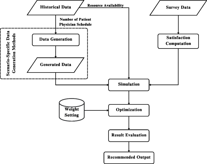
Scenario-driven resource optimization framework for sustainable hospital operations

The framework focuses on optimizing two key outcomes: patient satisfaction measured by metrics such as length of stay and physician assignment, and resource allocation by balancing staff and equipment levels with operational costs to achieve sustainable hospital operations.

The multi-objective optimization within this framework provides decision-makers with practical strategies to address both present and future challenges. By anticipating various scenarios, the framework ensures that hospitals remain resilient, efficient, and aligned with the SDGs, particularly SDG 3 (Good Health and Well-Being), SDG 10 (Reducing Inequalities), and SDG 11 (Sustainable Cities and Communities).

Data generation techniques and case study design

To capture the effects of external shifts, such as population aging, pandemic disruptions, and increased referral demands, this study defines a set of deterministic scenarios with structured adjustments to key parameters. These scenarios allow decision-makers to explore system performance under diverse but plausible operating conditions. However, it is important to note that random variation and probabilistic uncertainty are not explicitly modeled; instead, the focus is on providing practical, scenario-based insights to support strategic hospital planning.

The ophthalmology department was selected as the focus of this study due to its high patient demand and the complexity of its clinical workflow, which involves multiple diagnostic and pre-consultation procedures. As one of the most frequently visited specialties, particularly by elderly patients, ophthalmology presents significant challenges in terms of resource coordination, patient flow management, and service efficiency. These characteristics make it an ideal case for evaluating the effectiveness of resource planning strategies. Moreover, because of its structured yet intricate operational processes, the ophthalmology department serves as a representative benchmark for other OPDs offering insights that can be adapted to improve service delivery across various clinical specialties.

The data collection consists of two type of data. First is real or historical data including patient visits, physician schedules, and resource availability, is gathered from ophthalmology departments in public hospitals. This data provides a baseline for understanding current operations. Another is simulated data. Scenarios are generated to explore future challenges. The three key scenarios are: Aging Society (a growing elderly population increases demand for eye care services), Pandemic Scenario (disruptions such as staff shortages and reduced patient visits impact hospital capacity), and Referral Acceptance Enhancement (ensuring the hospital can accept more referrals from smaller or rural facilities despite resource constraints). This combination of real and simulated data ensures that the framework accounts for both present-day operations and potential future disruptions.

Scenario 1: aging society

In the aging society scenario, the focus is on modeling the anticipated increase in patients requiring healthcare services due to age-related conditions. As populations age, the demand for specialized care is expected to rise significantly. To make this framework adaptable to different environments, it is important to observe statistical trends in population growth over the next decade to assess changes in age demographics. This involves computing the percentage shift in population for various age ranges using demographic projections and historical data as shown in Fig. 3.

Resource planning framework for aging society scenario

The framework assumes that changes in the percentage of a specific age group within the population directly correlate with changes in the number of patients from that age group seeking healthcare services. For example, if the population aged 65 years and older constitutes 15.9% of the total population in 2025 and is projected to increase to 22.7% by 2035, the percentage shift in this age group is 6.8%. Under this assumption, the patient volume for this age group is also expected to increase by 6.8%. This percentage shift is then applied in the simulation model to adjust the incoming patient volume.

The goal of this scenario is to determine the optimal resource allocation needed to maintain high patient satisfaction, particularly concerning LOS and physician assignment, while minimizing the additional costs of hiring more physicians or purchasing equipment. Resource constraints are also set within the model to prevent over-hiring and maintain operational sustainability. By running the simulation with this projected patient increase, we can estimate the number of physicians and equipment required to deliver high-quality care to a growing elderly population while balancing costs.

Scenario 2: pandemic scenario

The pandemic scenario models the operational disruptions and adjustments required during a healthcare crisis, such as those experienced during the COVID-19 pandemic. This includes changes to patient flow, adjustments to resource availability, and the addition of patient triage processes to identify critical cases and manage infection risks. In this scenario, as shown in Fig. 4, the patient intake process is modified to include a triage step, which filters patients based on their condition. Patients requiring immediate medical attention are redirected to the emergency department rather than being admitted to regular outpatient services. This ensures that resources are allocated efficiently while minimizing exposure risks. Additionally, to comply with health and safety regulations—particularly social distancing guidelines—the number of available resources is deliberately reduced. This constraint helps enforce spacing between patients and prevents overcrowding in service areas, reflecting real-world restrictions implemented during pandemic periods.

Resource planning framework for pandemic scenario

During a pandemic, healthcare providers face unique challenges, particularly with physician availability. Some physicians may be directly affected by the pandemic, such as falling ill themselves, while others may be reassigned to support critical areas like the emergency department or community outreach teams. This creates a shortage of physicians in outpatient services, which must be accounted for in the resource constraints of the model. For instance, a 40% chance of unavailability means that on any given day, there is a 40% probability that a physician cannot work in the outpatient department due to illness or reassignment. This variability is incorporated into the model as an adjustable constraint to reflect the unpredictable nature of workforce disruptions during a crisis.

Additionally, the model accounts for the increased complexity of processes typically introduced during pandemics. The inclusion of additional triage steps, for example, ensures that patients are appropriately categorized based on the severity of their condition. By incorporating these adjustments, the framework use to identify the necessary resource levels—such as the number of triage stations, physicians, and support staff—needed to maintain service quality. The output provides actionable insights into balancing patient satisfaction, staff workload, and resource constraints under pandemic conditions, enabling hospitals to plan effectively for future crises.

Scenario 3: referral acceptance enhancement

The referral acceptance enhancement scenario focuses on addressing the challenge faced by large hospitals in urban areas that receive referral cases from smaller, rural hospitals with limited equipment and resources. These referral cases often involve patients who require specialized care or urgent medical attention that cannot be provided by their local healthcare facilities. The problem arises when large hospitals, due to resource constraints, are unable to accept a significant portion of these referrals, leading to delays in treatment and inequalities in healthcare access.

To address this issue as shown in Fig. 5, it is essential to first determine the hospital’s current referral acceptance rate and engage with decision-makers to establish a target acceptance rate that aligns with the hospital’s capacity and healthcare goals. For example, if the current acceptance rate is 20%, the hospital may aim to increase it to a more equitable and feasible level, such as 40% or 50%, depending on resource availability and patient demand. This target rate is then incorporated into the model as an adjustable parameter, allowing for scenario-specific analysis.

Resource planning framework for referral acceptance enhancement scenario

In the model, referral cases are assigned a higher priority to reflect their urgency and ensure they are addressed promptly upon arrival. The simulation explores the additional resources required—such as physicians, support staff, and equipment—to achieve the desired referral acceptance rate without compromising care for other patients. Constraints are applied to balance resource investments with operational efficiency, ensuring that the hospital can handle the increased volume of referrals sustainably. The resulting insights provide a strategic resource plan that enables the hospital to improve referral acceptance, thereby enhancing access to specialized care for underserved populations and contributing to the reduction of healthcare inequalities.

Satisfaction computation

The satisfaction survey used in this study is divided into three parts, designed to gather comprehensive data on patient demographics, satisfaction related to LOS, and preferences for physician assignment.

• General Information: The first part collects basic demographic and usage information, including the patient’s age, gender, and frequency of hospital visits. This data provides context for understanding patient satisfaction across different population segments.

• Satisfaction Related to LOS: The second part focuses on patient satisfaction with their time spent in the hospital. Patients are asked to rate their overall satisfaction on a scale from 1 (very unsatisfied) to 5 (very satisfied) for their most recent hospital visit. Additionally, they are asked to rate their satisfaction for specific LOS intervals: less than 1 hour, 1–2 hours, 2–3 hours, and more than 3 hours. This approach captures how satisfaction varies with the amount of time spent in the hospital, providing detailed insights into the impact of LOS on patient experience.

• Satisfaction Related to Physician Assignment: The third part evaluates patient preferences and satisfaction regarding physician assignment. Patients indicate their preference for seeing a general physician or a specialist based on their symptoms. They also specify whether they have a strong preference for a particular physician type or if they are comfortable with any available physician. This data helps assess the alignment between patient expectations and the hospital’s ability to meet their needs.

This structured survey design allows for a detailed evaluation of factors influencing patient satisfaction and provides the foundation for computing satisfaction metrics used in the simulation and optimization framework.

Satisfaction related to LOS computation

This process involves generating a predictive function to estimate patient satisfaction scores related to LOS. The survey includes general information questions and satisfaction-related questions, where responses are either binary (for general information) or ordinal (for satisfaction with LOS).

To analyze this type of data, Ordinal Logistic Regression [70] is used as the statistical method to develop the predictive function for satisfaction scores based on influencing factors. All variables are incorporated into the ordinal logistic regression model using Minitab software. The resulting function estimates the cumulative probability of a patient assigning a satisfaction rating of j or lower, expressed as \(P(S \le j)\), where S represents the satisfaction level on a scale from 1 to 5. The model includes n explanatory variables, denoted as \(X_{1},…, X_{n}\), which influence patient satisfaction. The intercepts for each satisfaction level are represented by \(\alpha _j\), while the regression coefficients for each explanatory variable are denoted as \(\beta _1,…, \beta _n\). The following Eq. (1) provides a structured method for assessing how different factors impact patient satisfaction with LOS.

To compute patient satisfaction related to LOS in this study, an ordinal logistic regression model is applied to survey data collected from outpatient respondents. The dependent variable represents the expected satisfaction score, ranging from 1 (very unsatisfied) to 5 (very satisfied), based on the patient’s perceived satisfaction for a specific LOS interval. The independent variables, denoted as X1 to X6, are derived from responses to structured survey questions. X1 captures gender as a binary variable (male/female), while X2 represents age groups as categorical values (below 18, 18–24, 25–44, 45–64, and over 65). X3 and X4 are binary indicators reflecting the patient’s prior experience visiting the hospital and the department, respectively. X5 denotes whether the patient had an appointment (yes/no), and X6 represents the LOS interval, categorized as: less than 1 hour, 1–2 hours, 2–3 hours, and more than 3 hours. The model estimates the probability distribution of satisfaction scores based on these factors. An example of the prepared dataset used to train the logistic regression model is shown in Table 1, where each row corresponds to a patient and their respective factor values and satisfaction rating. Each patient provides their expected satisfaction score for each LOS interval, allowing the model to capture how satisfaction varies with different waiting times.

After fitting the survey data into the ordinal logistic regression model, the analysis yields the intercept values (\(\alpha _j\)) and regression coefficients (\(\beta _n\)) corresponding to the factors influencing patient satisfaction. These coefficients quantify the impact of each explanatory variable on the satisfaction score related to LOS. To apply this model within the simulation, each patient is assigned specific values for the influencing factors, which are then input into the predictive Eq. 1 to calculate the probability distribution across five possible satisfaction levels. The model includes multiple predefined probability sets, each corresponding to different combinations of influencing factors—such as a patient who has visited the hospital but not the department, or one who has visited both. Each of these combinations results in a distinct satisfaction probability profile. Notably, the LOS value calculated dynamically from the simulation is also a key input in determining which probability set is used, ensuring that the predicted satisfaction reflects both the patient’s background and their experience in the system.

Once these probabilities are generated, the simulation model uses them to assign a satisfaction score to each patient. For every individual, the model draws a random number \(\theta\) between 0 and 1, and compares it to the cumulative distribution of the satisfaction probabilities. The patient’s final satisfaction score related to LOS, denoted as \(PSLOS_p\), is determined based on the interval into which the random number falls. This process ensures that satisfaction outcomes are both data-driven and dynamically responsive to each patient’s characteristics and experience. As a result, the simulation can reflect realistic variability in satisfaction across different scenarios, enhancing the robustness and applicability of the model. The full process of computing \(PSLOS_p\) is illustrated as follows:

• \(PSLOS_p=1\),

  if \(\theta \le P(S_1)\)

• \(PSLOS_p=2\),

  if \(P(S_1) \le \theta \le P(S_1)+P(S_2)\)

• \(PSLOS_p=3\),

  if \(P(S_1)+P(S_2) \le \theta \le P(S_1)+P(S_2)+P(S_3)\)

• \(PSLOS_p=4\),

  if \(P(S_1)+P(S_2)+P(S_3) \le \theta \le P(S_1)+P(S_2)\)\(+P(S_3)+P(S_4)\)

• \(PSLOS_p=5\),

  if \(P(S_1)+P(S_2)+P(S_3)+P(S_4) \le \theta \le P(S_1)\)\(+P(S_2)+P(S_3)+P(S_4)+P(S_5)\)

Satisfaction related to physician assignment computation

This process involves developing a method to compute the expected satisfaction score related to physician selection. From survey, patients provide symptom names that can be overly specific or infrequent. To evaluate patient satisfaction related to physician assignment, it is essential to classify symptoms based on their severity and required level of medical expertise. In this study, symptoms reported by patients are grouped into three categories based on literature [71,72,73,74]: Easy, Varied, and Hard. This classification helps determine whether a general physician or a specialist is more appropriate for the patient’s condition, which in turn influences satisfaction expectations.

1. 1.

   Easy symptoms refer to conditions that are mild, self-limiting, and typically do not require specialized treatment. These symptoms can be effectively managed by a general physician, and patients with such conditions generally do not expect or require specialist consultation. An example of an easy symptom is a stye, which often resolves on its own within two weeks and requires only basic care or observation [75].

2. 2.

   Hard symptoms are conditions that are severe, chronic, or potentially sight-threatening, and typically require immediate attention from a specialist. Patients experiencing these symptoms expect to see a specialist physician due to the complexity and urgency of care needed. For instance, glaucoma is categorized as a hard symptom because it can lead to irreversible vision loss if not managed promptly by a specialist [75].

3. 3.

   Varied symptoms are those that fall between easy and hard. Their severity depends on the underlying cause, and the treatment may or may not require specialist care. These conditions might be managed by a general physician in some cases, but may require referral to a specialist in others. An example of a varied symptom could be eye redness, which might result from simple irritation or be a sign of a more serious condition like uveitis [75].

This classification approach ensures that patient expectations for physician type are contextually appropriate, and allows the model to realistically assess satisfaction based on whether the patient was matched with their expected level of care. Patients also express their expectations regarding physician assignment based on their symptoms. These expectations fall into three categories: satisfaction with seeing a general physician, satisfaction only if seen by a specialist, or no preference for either physician type. Using the collected data, the probability of each symptom being associated with a specific physician expectation is computed.

Once the patient meets a physician, three possible outcomes determine their satisfaction score:

• If the assigned physician matches the patient’s expectation, the satisfaction score is 2.

• If the assigned physician differs from the patient’s expectation, the satisfaction score is 0.

• If the patient has no physician preference, the satisfaction score is 1, regardless of the assigned physician.

This method is then applied in the simulation model, where the equation for patient satisfaction related to physician assignment for each patient p, denoted as \(PSPA_p\), is represented in (2). The expected physician for each patient is denoted as \(EXP_p\), while the actual assigned physician is represented as \(AP_p\).

, while \(i \in I\) is a specific physician type from the set of all physician types

Simulation and optimization process

Simulation

The framework employs DES to model patient flow and resource utilization within hospitals. This approach captures the complexity of healthcare workflows, including appointment scheduling, patient consultations, and diagnostic procedures. By simulating these dynamics, the framework predicts operational outcomes under different scenarios, helping hospitals assess resource efficiency and patient care quality.

Patient satisfaction serves as the primary metric for evaluating the framework’s effectiveness, with two key indicators: LOS which is the total time a patient spends in the hospital and Physician Assignment Satisfaction which whether patients are assigned to their preferred or expected physician. The DES model analyzes how different resource allocation strategies impact these metrics, offering data-driven insights for hospital decision-making.

In this study, we focus on modeling the OPD process flow, beginning from the moment patients arrive at the hospital. Upon arrival, each patient is required to scan their appointment card or ID to receive a queue number, marking the start of their journey through the OPD system. Patients then proceed to wait for triage, where a nurse assesses their condition and directs them to the appropriate next steps. The triage process operates based on queue priority, with patients categorized into four types: Type A (appointments between 9:00–10:00 AM), Type B (10:00–11:00 AM), Type C (11:00–12:00 PM), and Type D (walk-in patients). Patients with earlier appointment times are given priority in the triage queue, while Type D (walk-in) patients are considered lowest priority. For the purpose of this simulation, it is assumed that emergency or urgent cases do not enter through the OPD.

To reflect realistic arrival behavior, the timing of patient arrivals is modeled using a time-dependent distribution derived from historical data. From the OPD’s opening at 7:00 AM until 9:30 AM, patient interarrival times follow a log-normal distribution with parameters LOGN(0.788, 0.447), capturing the peak arrival period. After 9:30 AM, the arrival pattern shifts to a Weibull distribution, defined as WEIB(4.89, 1.02), representing a gradual decline in patient inflow. All time units are expressed in minutes, and this dynamic modeling approach ensures that the simulation accurately mirrors real-world variability in patient arrival rates across the operating hours.

Following triage, patients wait to receive their personal medical file, which is handed out on a first-come, first-served (FCFS) basis according to the triage completion order. Once the file is received, the first mandatory pre-process for every patient is the Visual Acuity Test. After that, the necessity of further pre-processing steps is determined by the triage nurse. These optional tests include: Eye Tonometry Test, Auto-Refractometry Test, Dilation, Optical Coherence Tomography (OCT), Ophthalmic Imaging, Intraocular Measurement, and Visual Field Test, carried out in that specific sequence. Each of these stations also follows an FCFS queuing system, although not all patients are required to undergo every test. The processing time for each procedure is determined from empirical data collected at the hospital and follows a distinct statistical distribution specific to each station, ensuring the simulation reflects realistic variation in service durations.

Once pre-processing is complete, patients proceed to wait for consultation with a physician, which typically begins at 9:00 AM. The consultation queue operates under a priority-based policy according to the patient’s appointment type. Between 9:00 AM and 10:00 AM, Type A patients (with appointments in that hour) are given the highest priority. If time permits and no Type A patients are waiting, Type D (walk-in) patients may enter the queue. From 10:00 AM to 11:00 AM, Type A patients who arrive late still retain top priority, followed by Type B, and lastly Type D, again only if capacity remains. This priority queuing approach ensures that scheduled patients are seen in a timely manner while allowing flexibility to accommodate walk-ins when possible. The simulation is designed to reflect this full process on a weekly operational cycle, capturing patient flow, resource utilization, and potential bottlenecks across multiple working days. Figure 6 illustrates the simulation model developed using Arena, which replicates the OPD workflow of the ophthalmology unit. The simulation was implemented using Arena software, supported by a licensed version provided through Sirindhorn International Institute of Technology (SIIT), Thammasat University.

Simulation model layout in arena software

To ensure the accuracy and reliability of the simulated outpatient process described above, the next step involves a thorough verification and validation of the model. Model verification aims to confirm the correctness of the model’s logic, while model validation assesses the model’s accuracy in representing the real system. Verification involves testing the model under extreme conditions, such as when only one patient enters the system, with all processing times set to constant values. The LOS serves as a key performance indicator in this process. To verify the model, the LOS generated by the simulation is compared with a manually calculated LOS, which is the sum of all processing durations under the assumption of no queuing delays. In this study, the calculated LOS was 78 minutes, which matched exactly with the LOS produced by the simulation. This confirms that the simulation logic is implemented correctly and aligns with the underlying assumptions of the model.

For validation, the model’s output, which is patient satisfaction related to LOS, is compared against actual patient satisfaction data collected via a survey. An independent two-sample t-test was conducted to evaluate whether the mean satisfaction scores from the simulation and real-world survey data differed significantly. Prior to the test, the distribution shapes and variances of the two datasets were assessed and found to be reasonably similar (standard deviations: 0.865 for observed, 0.675 for simulated). When the ratio of standard deviations is less than 2, the assumption of equal variances is acceptable for a two-sample t-test [76], supporting the use of this method in our analysis. Both datasets comprised 300 samples. According to Van Voorhis and Morgan [77], a sample size of 30 or more per group is typically adequate to detect medium effect sizes with reasonable power in t-tests. The t-test yielded a p-value of 0.113, which is greater than the 0.05 threshold, indicating no statistically significant difference between the two groups. This result supports the validity of the simulation model in accurately reflecting real-world patient satisfaction trends. Together, the verification and validation processes demonstrate that the simulation model is both logically and realistically representative of the actual hospital system, making it suitable for further scenario analysis and decision support.

Optimization

To achieve optimal results, the framework integrates multi-objective optimization, specifically the TH approach, to balance competing goals: maximizing patient satisfaction with LOS, improving physician assignment satisfaction, and minimizing resource costs. Optimization tools such as OptQuest are used to identify effective resource allocation strategies while maintaining operational constraints. The framework also evaluates trade-offs between increasing staff or equipment and associated costs, providing adaptable solutions tailored to hospitals of varying capacities.

The optimization model is based on key assumptions to ensure practicality. It assumes that increasing resources (e.g., physicians and equipment) directly enhances patient satisfaction by reducing LOS and improving physician assignment alignment. Resource allocation is modeled within budget constraints, allowing for the exploration of different configurations. Additionally, a linear relationship between resource levels and costs is assumed to simplify real-world complexities and ensure computational efficiency. These assumptions enable the framework to balance trade-offs between patient satisfaction and cost-effectiveness, offering hospitals a structured approach to sustainable resource management.

The notation used in the following optimization model is summarized in Table 2. The length of stay for each patient (\(LOS_p\)) is calculated using Eq. (3), which considers queuing delays based on current and additional physician and resource levels, as well as individual patient service and transfer times. This calculated LOS value is then used to derive the satisfaction score related to LOS (\(PSLOS_p\)) through an ordinal logistic regression in Eq. 1.

The decision variables in the optimization model include the number of additional physicians (\(D_i\)) and the amount of each additional resource (\(M_j\)). The objective functions, derived from [30], are designed to achieve three key goals: maximizing patient satisfaction related to LOS (\(Z_1\)), maximizing patient satisfaction with physician assignment (\(Z_2\)), and minimizing investment costs (\(Z_3\)). These objectives are explicitly defined in Eqs. (4)–(6).

The model incorporates constraints to ensure practical feasibility. Specifically, the number of additional physicians cannot exceed the maximum allowable limit, as defined in Eq. (7). Similarly, the allocation of additional resources must remain at or above the current levels while not exceeding the maximum allowable limit, as described in Eq. (8). By integrating these constraints, the optimization framework balances patient satisfaction and cost-effectiveness while adhering to real-world hospital capacity limitations.

Objective function:

Subjected to:

The objectives of maximizing patient satisfaction related to LOS, maximizing satisfaction with physician assignment, and minimizing investment costs inherently conflict with one another. The three objectives in this study inherently conflict with one another. Maximizing patient satisfaction related to LOS (Eq. 4) often requires allocating additional physicians and resources, which increases overall operational cost (Eq. 6). Similarly, maximizing satisfaction with physician assignment (Eq. 5) may involve assigning specific physician types based on patient preferences, potentially increasing staffing needs or limiting scheduling flexibility. These trade-offs reflect the practical challenge in balancing service quality and financial constraints in outpatient department planning. To address this challenge, the multi-objective optimization framework balances these competing goals by incorporating fuzzy linear programming and weight sets, ensuring that decision-makers can evaluate trade-offs effectively. This structured approach leads to robust and adaptive solutions that align with real-world hospital constraints, promoting sustainable and efficient resource allocation.

Multi-objective optimization involves solving multiple objective functions simultaneously, with each assigned a level of importance using weight factors, denoted as \(w_o\), for each objective o. However, based on in-depth interviews with hospital experts, it was determined that specific weight assignments could not be predefined, as all objectives were considered equally important. To maintain flexibility, the weight settings needed to be adjustable. Since expert-defined preferences were unavailable, a set of twenty-five weight configurations was adopted as recommended by [78]. Each configuration includes weight distributions for both patient satisfaction objectives and investment cost minimization, as detailed in Table 3. Utilizing multiple weight settings provides significant advantages in multi-objective optimization, allowing decision-makers to explore different prioritization scenarios. By evaluating various weight combinations, hospitals can assess a range of possible outcomes, ensuring that resource allocation aligns with their specific needs and situational constraints while maintaining a balanced approach to patient satisfaction and cost efficiency.

To perform multi-objective optimization, this study employs the Torabi-Hassini (TH) approach for fuzzy multi-objective optimization, as proposed by Torabi and Hassini [79]. This method is particularly well-suited for decision-making in uncertain environments, offering a flexible, robust, and interactive framework for balancing multiple competing objectives. Unlike traditional fuzzy optimization techniques, the TH approach integrates procurement, production, and distribution into a single model, allowing for compromise solutions that improve practicality for decision-makers seeking a fair trade-off between conflicting goals.

To solve the multi-objective optimization problem using the TH approach, the objective functions \(Z_o\) for each objective o are first defined. Next, the positive ideal solution (PIS) and negative ideal solution (NIS) for each objective function are determined by solving the corresponding mixed-integer linear programming (MILP) model individually. The PIS for each objective o, denoted as \(Z_{o}^{PIS}\), represents the best possible outcome, while the NIS, denoted as \(Z_{o}^{NIS}\), represents the worst possible outcome. Once these values are established, a linear membership function is specified for each objective function as follow:

For Minimize Objective:

For Maximize Objective:

, where \(\mu _o(v)\) represents the satisfaction degree of the oth objective function. The auxiliary multi-objective MILP model is then transformed into an equivalent single-objective MILP using the auxiliary crisp formulation given in Eq. 11.

Auxiliary MILP:

subjected to:

, where \(\lambda _h = \min _o{\mu _o(v)}\) represents the minimum satisfaction degree among all objectives. The parameter \(\gamma\) acts as a compensation coefficient, controlling the minimum satisfaction level of objectives and implicitly determining the degree of compromise among them. This value can be adjusted based on the desired balance between competing objectives. A higher \(\gamma\) leads to a more balanced compromise solution, ensuring that all objectives are fairly considered. Conversely, a lower \(\gamma\) prioritizes one objective with minimal regard for the others. In this study, \(\gamma\) is set to 0.4 to achieve a balanced trade-off among objectives. Finally, the auxiliary crisp model (11) is solved under the given constraints (12), (13), and (14).

The following algorithm outlines the multi-objective optimization procedure used in this study. The process iteratively evaluates combinations of decision variables, specifically the number of physicians and medical equipment, under varying weight sets for the three objectives: maximizing satisfaction related to LOS, maximizing satisfaction related to physician assignment, and minimizing cost. The algorithm first runs single-objective simulations to establish positive (PIS) and negative (NIS) points. It then performs optimization across 25 weight configurations using the Torabi-Hassini (TH) approach. For each weight set, the simulation model is executed, and the resulting objective values are normalized and aggregated to identify the optimal policy. Figure 7 serves to illustrate the structured flow of this optimization process.

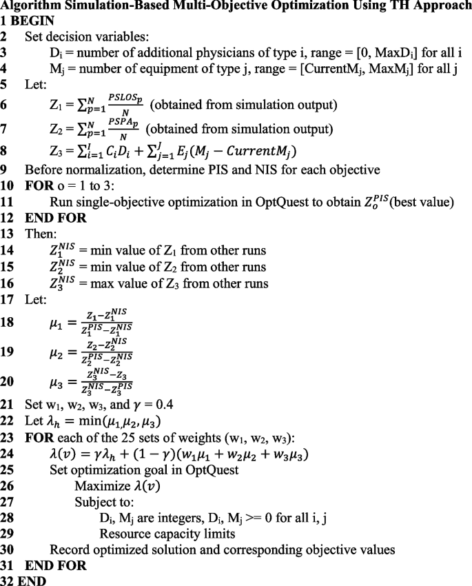
Simulation-based multi-objective optimization algorithm using Torabi-Hassini approach and OptQuest

Evaluation of results and recommendation process

After performing the optimization, the objective values of the optimized solutions are collected, including the average satisfaction scores related to LOS, physician assignment satisfaction, and cost. These values are then analyzed to determine whether significant differences exist across different optimization weight configurations. To evaluate these differences, Analysis of Variance (ANOVA) and Tukey’s test are applied. Each weight configuration is referred to as a case, with a total of 28 cases considered.

The analysis examines multiple factors, including cases and replications, with replications treated as a blocking factor. The responses measured include patient satisfaction scores for LOS and physician assignment, which are analyzed separately. Using ANOVA, the null hypothesis assumes that the average satisfaction scores across all cases are equal, while the alternative hypothesis suggests that differences exist. A 95% significance level is used, meaning that if the p-value is \(\le\) 0.05, the null hypothesis is rejected. The results confirm that satisfaction scores vary across cases, necessitating further analysis using Tukey’s test.

Tukey’s test is employed to reorganize the data and identify the highest satisfaction scores by comparing all pairs of means. It groups satisfaction scores that do not show statistically significant differences. All statistical analyses are conducted using Minitab 20.

Following the grouping process, the base case serves as a benchmark for comparison. Cases are categorized based on their satisfaction scores relative to the base case:

• “Higher” – Case with significantly higher satisfaction scores than the base case.

• “Unchanged” – Case within the same statistical group as the base case.

• “Lower” – Case with significantly lower satisfaction scores than the base case.

This classification helps in identifying the most effective resource allocation strategies for improving patient satisfaction across different hospital scenarios.

The decision guideline logic is developed through a comprehensive evaluation of each event’s impact on patient satisfaction and investment costs, serving as a critical decision-support tool for hospital resource management. These guidelines are designed to help decision-makers identify and prioritize events that effectively enhance patient satisfaction while ensuring cost-effectiveness. The decision logic is structured as follows:

1. 1.

   Case with Both Lower: If both satisfaction metrics (LOS and physician assignment) are labeled as “Lower”, the case is not recommended. This indicates that implementing the case would result in a decline in patient satisfaction for both factors, making it an unsuitable option.

2. 2.

   Case with One Lower and One Unchanged: If one metric is “Lower” and the other is “Unchanged”, the case is not recommended. Without any improvement in either objective and a decline in one, adopting this case would not be beneficial.

3. 3.

   Case with Both Unchanged: If both satisfaction metrics remain “Unchanged”, the case is not recommended. Since no improvements are observed, implementing such a case would not provide meaningful benefits to the hospital system.

4. 4.

   Case with Both Higher: If both satisfaction metrics are labeled as “Higher”, the decision should consider investment cost. If the cost falls within an acceptable range set by hospital decision-makers, the case is recommended. However, if the cost exceeds the acceptable threshold, the case should be compared with other alternatives to ensure cost-effectiveness.

5. 5.

   Case with One Higher and One Unchanged: When one satisfaction metric is labeled as “Higher” and the other as “Unchanged”, the investment cost becomes the deciding factor. The case with the lowest investment cost is recommended, as it provides an improvement in at least one objective while maintaining the other without unnecessary expenditure.

6. 6.

   Case with One Higher and One Lower: If one metric is labeled as “Higher” and the other as “Lower”, the case is not recommended. A decline in one satisfaction factor outweighs any potential gains in the other, making this case an unsuitable choice.

This framework provides hospitals with a powerful tool to anticipate and manage resource needs proactively. It equips decision-makers with actionable insights into patient satisfaction, resource allocation, and operational efficiency, aligning with the SDGs to support sustainable healthcare development.