
Decarbonization pathways in medical waste management through circular economy strategies to advance UN-SDGs

In this paper, a strategic evaluation scheme is advocated for decarbonization trajectories over MWM, and it incorporates the CE principles with the MCDM techniques under uncertainty. The process can be segmented into a series of steps and is presented as follows:
Application of the methodology
Specific to practical relevance, the framework was employed on Pakistani medical and healthcare setting varying in terms of size and resource capacity. The collected data were used to formulate criteria for evaluation and CE initiatives, and MCDM methodologies were applied to evaluate the performance of various interventions under uncertainty. The results were benchmarked against UN-SDGs aimed at demonstrating sustainability improvements. The application demonstrated the optimal and practical CE strategies in hospitals and healthcare centers, confirmed the good effectiveness of the stimulus framework for CE-MWM capacity based on evidence and decarbonized approach prosecution.
Study framework and ANP-DEMATEL techniques
The ANP-DEMATEL method combines the capabilities of the Analytic Hierarchy Process, Decision-Making Trial and Evaluation, and the Analytic Network. The DEMATEL method which making it possible to analyze and calculate an influence matrix, clarifying the strengths, intensity by among reciprocal cause-and-effect connections. Not all factors can in reality affect the entire system uniformly, so that each factor does not have the same weights40. Second, utilizing the network structure of determining elements by the DEMATEL method, and finally we apply it to adjust factor weights with ANP approach in a more general condition. To ensure adherence to ethical principles, we obtained official written approval from the Research Ethics Committee of the School of Business at Xian International University. Written consent was obtained from all participants, who were guaranteed anonymity. Finally, we told participants that the data would be used only for academic purpose and no private information would be revealed.
DEMATEL & ANP approach calculation procedure
DEMATEL-ANP methodology is commonly applied for the priority assessment of criteria focusing on the intricacies and interactions between different parameters41,42. The DEMATEL-ANP method has been used in many kinds of research studies such as financial decision making, supplier selection, and sustainable exploration like medical waste management systems43,44,45. This study aims to explore the intricate interrelationship and prioritization of medical waste drivers. Insight into method maturity, this study can proficiently utilize the DEMATEL-ANP scheme. Therefore, the DEMATEL-ANP conducts a structural causal analysis and a scan of significant enablers. The comprehensive framework of this research is developed using the DEMATEL-ANP technique, as shown in Fig. 1. Here, we detail the method’s comprehensive calculation, data collection, and processing.

Study Framework and ANP-DEMATEL approach.
The DEMATEL calculation process
DEMATEL solves intricate system problems by developing structural models to indicate the influence relations among several factors46. In this way, graph theory and matrix techniques are used for index analysis, and a direct influence matrix is constructed from the influence relations among factors. Subsequently, each factor’s central and causal degree is computed, and a diagram is developed. The causal ties between factors and their relative importance within the factor system are determined47,48. The calculation procedure is described as follows.
Construct the direct effect matrix and normalize
In the DEMATEL approach, experts assess the direct impact of the factor i on factor \(j~\)on a scale from 0 to 4, where 0 indicates “no influence” and 4 indicates “very high influence,” show in Table 2. The degree of contribution is represented as \(dij\), and we average the score of each expert on this pair of attributes to obtain the direct influence average matrix A, which can be formulated as:
$$A=\left( {\begin{array}{*{20}{c}} 0&{{a_{12}}}& \ldots &{{a_{1n}}} \\ {{a_{21}}}&0& \ldots &{{a_{2n}}} \\ \vdots & \vdots & \ddots & \vdots \\ {{a_{n1}}}&{{a_{n2}}}& \cdots &0 \end{array}} \right)$$
(1)
Here \(aij\) is the mean of \(dij\), which is the mean score for i influencing \(j.~\)Because a component cannot have any effect on itself, the diagonal elements \(\left( {~aii} \right)\) are all zero. Let A be the matrix representing the direct impact relations between the system factors.
According to Eqs. (2) and (3), the matrix A is then normalized based on the column and row normalization to gain a normalized direct influence average matrix X, and each factor of X falls in the range (0, 1).
$$Min\left[ {\frac{1}{{\mathop {{\text{max}}}\limits_{{1 \ll i \ll n}} \mathop \sum \nolimits_{{j = 1}}^{n} \left| {a_{{ij}} } \right|}},\frac{1}{{\mathop {\max }\limits_{{1 \ll j \ll n}} \mathop \sum \nolimits_{{i = 1}}^{n} \left| {a_{{ij}} } \right|}}} \right]$$
(2)
Construct the comprehensive influence matrix T
The Eqs. (4) and (5) compute the total impact matrix T.
$$\begin{array}{*{20}{c}} {T={{\left[ {{t_{ij}}} \right]}_{n \times n}},i,j \in \left\{ {1,2,3, \cdots n} \right\}} \end{array}$$
(4)
$$T=X{(I – X)^{ – 1}}$$
(5)
Here, \(I~\)is devoted to the unit matrix, and inside the T matrix, the summation of \(ith\) the row indicates the aggregate direct and indirect effects attributable to the factor \(\:i\) on other factors. Likewise, inside the T matrix, the summation of \(\:jth\:\)column represents the aggregate direct and indirect impacts derived by the factor \(\:j\:\)from other factors.
Determine the center degree and rationale degree of each element
In the total influence matrix, the sum of all values in a row is used to measure the factor’s total direct and indirect effects on other factors (Eq. 6), which is called the influencing degree (R). In contrast, the sum of the column gives the overall impact that factors from the other parts of the system (Eq. 7), which is called the influenced degree (C). These measures then calculate every factor’s center degree and cause degree. The center degree represents a factor’s overall importance in the system (the higher the importance, the stronger interactions it tends to have with the other elements). If its value is greater than 0, its impact overrides all other factors and becomes the cause factor. When its value is less than 0, other factors influence the factor more and are designated as the resulting factor. The cause-and-result factors can be easily understood by applying the degree: a positive value denotes a cause factor that affects most other factors. In contrast, a negative value denotes a result factor affected most by other factors in the system. These values indicate the importance, as well as the direction, of the impact within the structural model.
$$\begin{array}{*{20}c} {R = \mathop \sum \limits_{{j = 1}}^{n} t_{{ij}} } \\ \end{array}$$
(6)
$$C = \mathop \sum \limits_{{i = 1}}^{n} t_{{ij}}$$
(7)
Create the influence diagram
The influence graph underlines the logical connections among elements, with the horizontal axis as the center degree value and the vertical axis as the reason degree value. The elements are connected via their relations expressed in the influence figure.
Computation of ANP
The ANP approach is an advanced version of AHP, developed for complex decision-making and introduced by Saaty in 199649. ANP can accommodate a non-independent hierarchical structure, precise assessment, and the prioritization of indicators at all levels by accounting for dependencies among clusters and factors50. ANP computation steps are concise by47, which are below.
ANP network structure development
The network structure of ANP describes the interconnections among factors across different hierarchies, displaying these interrelations using bidirectional arrows or arcs47. The formulation of the ANP network structure based on identified factors and their interconnections, derived from the DEMATEL influence diagram using Super Decision software and Excel.
Pairwise comparison matrix development
The pairwise comparison matrix was developed by following Satay’s consistent matrix approach. Experts for this study were requested to evaluate the relative significance of factors within the same structure via pairwise comparisons using a nine-point Saaty scale, as shown in Table 3. Through pairwise assessment of relatively significant elements, a matrix was developed, which is devoted to a pairwise comparison matrix.
Consistency check
CR (Consistency Ratio) and CI (Consistency Index) are used to check the pairwise comparison matrix consistency logically by using Eqs. 8 and 9. The \(CR\) of pairwise comparison < 0.1 is logically reliable.
$$\begin{array}{*{20}{c}} {CI=\frac{{{\lambda _{max}} – {\text{n}}}}{{{\text{n}} – 1}}} \end{array}$$
(8)
$$CR=\frac{{CI}}{{RI}}$$
(9)
Where n represents the pairwise comparison matrix size, while λmax signifies the pairwise comparison’s maximum eigenvalue, and \(RI\) is the average value of the stochastic matrix \(CI~\)with \(RI\) from ranging value at 0.00, 0.58, 0.90, 1.12, 1.24, 1.32, 1.41, 1.45, 1.51 for \(n=\) 2,3,4,…,1 respectively
Develop the unweighted super-matrix
The pairwise comparison matrix outcomes are used to construct an unweighted super-matrix W’. Equation 10 defines its mathematical formulation of super-matrix W’.
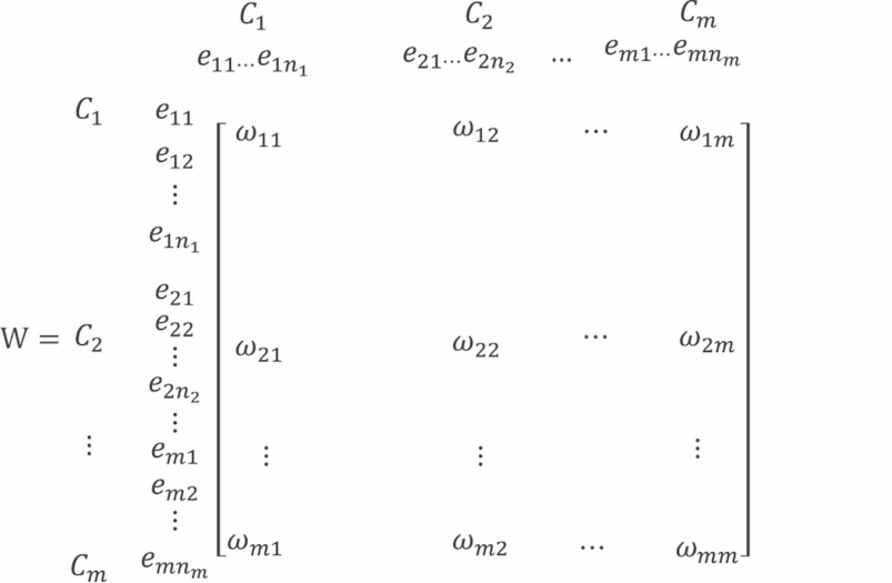
(10)
In the above context, m is defined as the clusters, while n signifies the factors quantity within every cluster. Same as \(cm\) represents the mth cluster, and mn indicates mth element in \(mn\)th cluster, and nm shows all the factor quantities in the math cluster. The equation \(\omega ij~\left( {\omega 11~.~.~.~\omega m1~.~.~.~\omega mm} \right)\) is represented by an unweighted super-matrix \(W{\prime }\), where \(\omega ij\) describes the eigenvector associated with the factors influencing in cluster ith on the\(~j\)th cluster’s factors, such as factors confined to primacy in the pairwise comparison. If there is no influence exists in the relationship, then \(\omega ij\) equals 0.
Derive the weighted super-matrix
It is essential to accurately assess indicators at a multi-level for deriving the weighted super-matrix because the unweighted super-matrix is developed without taking influences among clusters. Equation (11) utilizes cluster taking as a variable and compares relative weights pairwise to construct a relative weight matrix C. Consequently, the weighted super-matrix W is developed by applying Eq. (12) by combining the relative weight matrix C and unweighted super-matrix W
$${\mathbf{C}}=\left[ {\begin{array}{*{20}{c}} {{c_{11}}}&{{c_{12}}}& \cdots &{{c_{1m}}} \\ {{c_{21}}}&{{c_{22}}}& \cdots &{{c_{2m}}} \\ \vdots & \vdots & \vdots & \vdots \\ {{c_{m1}}}&{{c_{m2}}}& \cdots &{{c_{mm}}} \end{array}} \right]$$
(11)
where \(cij\) denotes the eigenvector value of influence of the cluster \(ith\) on cluster \(jth~\)such as the clusters’ primacy in the pairwise comparison.
$${{W^{\prime} = }}\left[ {\begin{array}{*{20}c} {\omega _{{11}} c_{{11}} } & {\omega _{{12}} c_{{12}} } & \cdots & {\omega _{{1m}} c_{{1m}} } \\ {\omega _{{21}} c_{{21}} } & {\omega _{{22}} c_{{22}} } & \cdots & {\omega _{{2m}} c_{{2m}} } \\ \vdots & \vdots & \vdots & \vdots \\ {\omega _{{m1}} c_{{m1}} } & {\omega _{{m2}} c_{{m2}} } & \cdots & {\omega _{{mm}} c_{{mm}} } \\ \end{array} } \right]$$
(12)
Obtain the limit super-matrix
For factor weights to be ascertained, Eq. (12), the weighted super-matrix is elevated to the power of \(\:k\) in Eq. (13) until stability is achieved. In the limited super-matrix, factors’ weights are located in respective columns, while the clusters’ weights indicate the total factor weights they encompass. The clusters and factor weights calculation are used to determine their priorities.
$$\mathop {{\text{lim}}}\limits_{{k \to \infty }} {\omega ^{2k+1}}$$
(13)
Acquisition of data and process
The DEMATEL technique does not require a large sample size, which can be used to analyze the interactions among factors simply51. Similarly, the ANP model does not impose a preset sample size; a study with a small sample size (N ≤ 30) is thought feasible in methodology52,53. In recent years, the ANP and DEMATEL approaches have been increasingly employed in small sample-size studies53,54. In the present study, we used a purposive sampling strategy to identify experts who could provide insightful views. Fifteen experts were invited to the DEMATEL and ANP analyses through questionnaires. These represent experts from four core segments in Pakistan: (1) government, (2) medical industry associations, (3) hospitals and healthcare centers, and 4) colleges and universities of medicine. The 10 experts with more than 10 years of working experience in sustainable medical management and participating in low-carbon medical supplies projects were selected. Panel of 5 to 10 experts in MCDM context has been used in healthcare/sustainability domains in some past studies such as55,56,57,58. Their practical and theoretical knowledge of low-carbon development in the medical and healthcare sector enhanced the accuracy and reliability of the research findings. A detailed description of the experts is given in Table 4. The two rounds of questionnaires were collected between January and March 2025. The DEMATEL questionnaire was provided on-site or by e-mail in the first round, and eight experts answered on-site and two answered by e-mail. Using a five-point Likert scale, this survey assessed the influence of relations between the detected driving factors. After establishing these relationships, the second round of the ANP questionnaire was conducted, which included estimating the subjective importance of the degrees of factors on a scale from Saaty’s nine-point scale. The panel of experts had responded to a similar questionnaire. The reliability analysis for the data obtained from the DEMATEL and the ANP was performed individually for consistency and reliability. To verify the data collected from the DEMATEL questionnaire, the responses of 10 experts were randomly and equally divided into two sets. A variance test was applied with SPSS software, yielding a p-value > 0.05 for each driver, meaning the two datasets are not statistically different. About the ANP questionnaire, consistency ratio (CR) testing was carried out with the aid of Super Decisions software, and the CR values were calculated according to Eqs. (8) and (9). All CR values were less than 0.1, indicating that the pairwise comparisons were internally consistent. Thus, data extracted from the DEMATEL and ANP questionnaires were considered acceptable and applicable for further investigation.
link


